> ./load-projects-NFL Data Bowl 2025-2025-11-14T00:00:00+00:00.sh
> loading progress bar...
[ ██████████████████████████████████████████████████ ] 100%> retrieving projects@November 14, 2025...
The NFL Data Bowl 2025 is an analytics competition hosted on Kaggle that focuses on analyzing NFL player tracking data. The competition challenges participants to develop machine learning models to predict various aspects of player performance and game outcomes using advanced data science techniques. The entire project is open source and available on my GitHub repository.
Datasets
The first thing to do in this competition is to try to understand the dataset and turn it into a format that can be used for training gomlx models. The data is in several csv files, each containing different types of information depending on the file name. If the filename starts with ‘input’ it contains the input data for the model. If it contains ‘output’ it contains the actual outcome for the data in the model.
Frames are recorded at a rate of 10 FPS. The coordinate system is as follows:
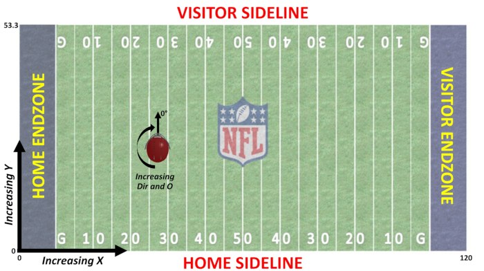
Coordinates used in the dataset. The origin is at the bottom left corner of the field. The x-axis runs along the length of the field, going from 0 at the end of the home team endzone to 120 at the end of the away team endzone. The y-axis runs across the width of the field with 0 at the home sideline and 53.3 at the away sideline. Left in the dataset refers to moving towards the hometeam endzone and right refers to moving towards the away team endzone. The angles are measured in degrees with 0 degrees pointing in the positive y direction and increasing clockwise.
The input data contains the following columns:
| Column Name | Description |
|---|---|
| game_id | Unique identifier for each game |
| play_id | Unique identifier for each play |
| player_to_predict | Unique identifier for the player whose performance is being predicted |
| nfl_id | Unique identifier for the player in the NFL database |
| frame_id | Frame identifier for each play. Starts at 1 for each game_id/play_id |
| play_direction | Direction offense is moving (left or right) |
| absolute_yardline_number | Distance to endzone for the offense |
| player_name | Name of the player |
| player_height | Height of the player in ft-in |
| player_weight | Weight of the player in lbs |
| player_birth_date | Birth date of the player |
| player_position | Position of the player |
| player_side | Side the player is playing on. (offense or defense) |
| player_role | Role of the player in the play (Defensive Coverage, Targeted Receiver, Passer or Other Route Runner) |
| x | x coordinate of the player on the field |
| y | y coordinate of the player on the field |
| s | Speed of the player in yards per second |
| a | Acceleration of the player in yards per second squared |
| o | Orientation of the player in degrees |
| dir | Direction of the player’s movement in degrees |
| num_frames_output | Number of frames to predict for the play |
| ball_land_x | x coordinate of the ball landing position |
| ball_land_y | y coordinate of the ball landing position |
Looking at this I’m probably going to want to implement the dataset based on the game_id and play_id, so that I can easily get all the data for a given play. I want to flag the player_to_predict and use that as the target for the model. So what I’m seeing is that the game will be a set of plays, each play will be a set of frames, and each frame will contain the data for all the players on the field at that time. I also don’t want to overwhelm the memory by loading all the data at once, so I will use a batched dataset that loads the data for a given play when it is needed. This way I can also easily implement data augmentation by randomly flipping the coordinates and angles for each play.
This should end up looking something like this:
type GameData struct {
    plays map[string]PlayData
}

type PlayData struct {
		PlayDirection string
		AbsoluteYardlineNumber float64
    Frames []frameData
}

type FrameData struct {
    Players []PlayerData
}

type PlayerSide uint

const (
    OFFENSE PlayerSide = iota
    DEFENSE
)

type PlayerRole uint

const (
    DEFENSIVE_COVERAGE PlayerRole = iota
    TARGETED_RECEIVER
    PASSER
    OTHER_ROUTE_RUNNER
)

type PlayerData struct {
    NflID string
    PlayerToPredict bool
    PlayerName string
    PlayerHeight float64
    PlayerWeight float64
    PlayerBirthDate time.Time
    PlayerPosition string
    PlayerSide PlayerSide
    PlayerRole PlayerRole
    X      float64
    Y      float64
    S      float64
    A      float64
    O      float64
    Dir    float64
}

type NFLDataBowl2025Dataset struct {
	InputData map[string]GameData
}
*** Probably unexported though ***
gomlx dataset
To work with gomlx, I will need to implement a gomlx.Dataset that can load the data for a given play in a format that can be used for training. This has to implement a specific interface, and to do batching I will need to implement a custom function to handle it. We’ll cross that bridge when the time comes.
I’ll need to be able to convert it to a flat train.tensor compatible
object. I’ll also need a way to batch the csv reads, so I don’t run out
of memory loading too many frames at once! This is all handled as part
of the dataset package.
Model
The model I’m using for this competition is the gomlx ‘simple’ model. It’s a model implemented in pure-go! The architecture is an MLP model that uses a basic ADAM optimizer.
Statistical Mechanics
The statistical mechanics method uses the training data to essentially build the forcefield the player particles experience, and use that to make predictions about where the players go next.
How it works:
- Index training data (lazy — only game_ids scanned at startup).
- Stream every training game through GameIter; extract empirical acceleration distributions into a ForceTable, grouped by (player_role, speed_bucket, dir_bucket).
- Load test rows from test_input.csv + submission template.
- For each test row, run -runs independent particle simulations starting from the player’s last observed kinematic state.
- Take the mean trajectory and read off the position at output frame N (frame_id/num_frames_output encodes which future step is requested).
- Write out/submission.csv with columns id,x,y.
Results
To compare the results, I wrote a command to compare the two methods. It
uses the dataset to train a model using the ml package as well as runs a
montecarlo simulation using the simulate package. In order to gauge each
model’s accuracy, I set aside some of the training data for use as
test data. I then was able to use that to compare not only each result
against eachother, but the results against a separately known value.
I ran my comparison command using
$ go run ./cmd/compare/ ... -epochs 10 -infer-batch 256 -runs 100
=== Prediction Accuracy Comparison (Euclidean distance, yards) ===

Method                N       MAE      RMSE     Median
------                -       ---      ----     ------
ML (MLP)      [all]   31637   3.7473   4.7710   2.9560
Monte Carlo   [all]   31637   1.1727   1.9834   0.5900

--- Early frames (1–5) ---
ML (MLP)      13690   2.8791   3.2652   2.6428
Monte Carlo   13690   0.2289   0.3334   0.1408

--- Mid frames (6–15) ---
ML (MLP)      15119   3.2715   3.8331   2.8671
Monte Carlo   15119   1.5507   1.9963   1.2032

--- Late frames (16+) ---
ML (MLP)      2828   10.4933   11.1572   10.1764
Monte Carlo   2828   3.7207    4.7080    3.1274

Winner (by MAE):
  All     Monte Carlo wins (ΔMAE = 2.5746 yds)
  Early   Monte Carlo wins (ΔMAE = 2.6502 yds)
  Mid     Monte Carlo wins (ΔMAE = 1.7208 yds)
  Late    Monte Carlo wins (ΔMAE = 6.7727 yds)
This shows that using only 10 epochs and a simple machine learning method, Monte Carlo makes better predictions.
Let’s see what happens when I crank it up to 40 epochs.
=== Prediction Accuracy Comparison (Euclidean distance, yards) ===

Method                N       MAE      RMSE     Median
------                -       ---      ----     ------
ML (MLP)      [all]   31637   3.7473   4.7710   2.9560
Monte Carlo   [all]   31637   1.1727   1.9834   0.5900

--- Early frames (1–5) ---
ML (MLP)      13690   2.8791   3.2652   2.6428
Monte Carlo   13690   0.2289   0.3334   0.1408

--- Mid frames (6–15) ---
ML (MLP)      15119   3.2715   3.8331   2.8671
Monte Carlo   15119   1.5507   1.9963   1.2032

--- Late frames (16+) ---
ML (MLP)      2828   10.4933   11.1572   10.1764
Monte Carlo   2828   3.7207    4.7080    3.1274

Winner (by MAE):
  All     Monte Carlo wins (ΔMAE = 2.5746 yds)
  Early   Monte Carlo wins (ΔMAE = 2.6502 yds)
  Mid     Monte Carlo wins (ΔMAE = 1.7208 yds)
  Late    Monte Carlo wins (ΔMAE = 6.7727 yds)
This took 20 minutes to calculate and had very little improvement. Monte Carlo appears to be winning every metric by a bit.
.> /load-comments-NFL Data Bowl 2025-linux-x64.sh